

Stringency index vs deaths in Covid-19: Country level analysis of Europe
Stringency index vs deaths in Covid-19: Country level analysis of Europe
All data come from covid.ourworldindata.org / focus on European countries

This is a follow up to my previous post: Stringency index vs deaths in Covid-19 Europe where i analyzed East vs West Europe “blocks” (log) daily variations in new deaths vs stringency index
The idea is to look into statistical relationships (or no relationships) between these 2 metrics
I will perform this analysis at country-level: Y = log of daily variations in new deaths per million and X = stringency index (lagged by 14 days)
I will provide scatter plot + linear fit (and R²) and results for coefficients from 30 days rolling window regressions
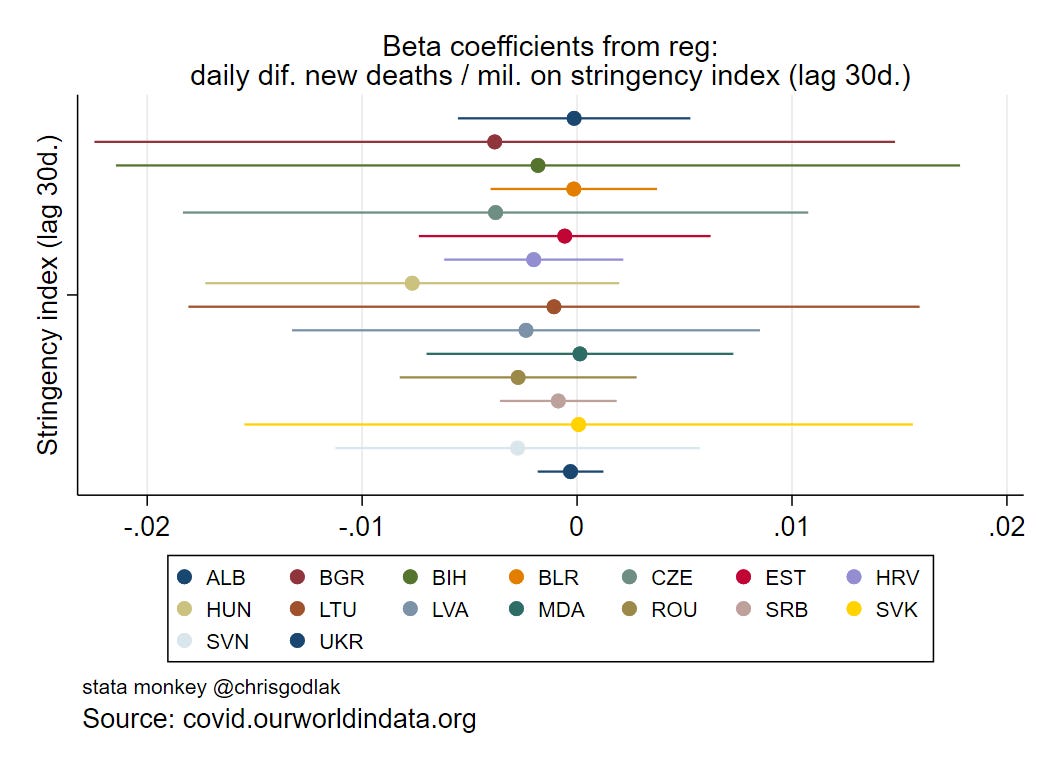
But first let me present you the coefficients’ plot for each country available: coefficients beta are the output from regressing Y on X (defined above) using OLS with robust standard errors; these are further used to plot the linear fits on the scatter plots hereafter
Remember that these coefficients are from regressing all observations; we obtain an “average” (linear by hypothesis) sensitivity measure for the whole year for each country
I present plots for East and West Europe:
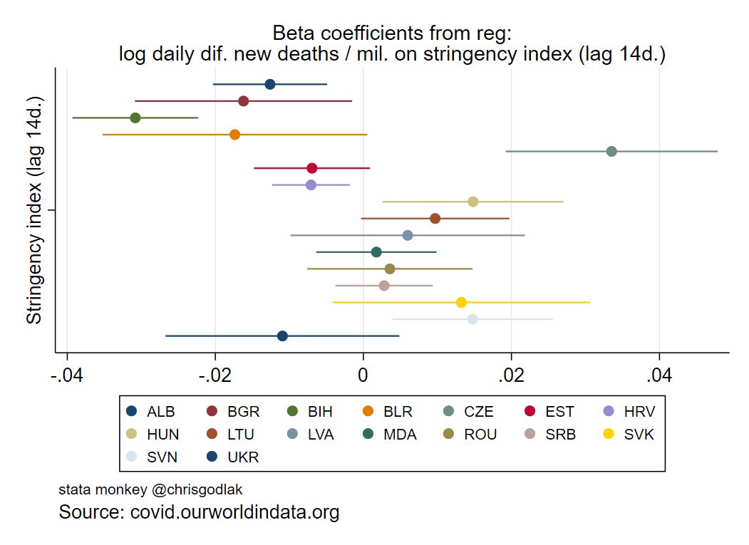
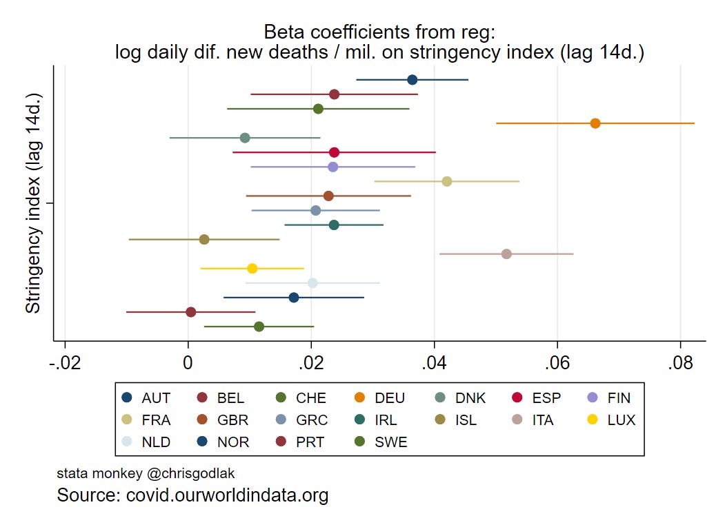
First of all, those coefficients are small in magnitude; mostly around 0. Some coefficients are < 0 (i.e. link between stringency & deaths is negative; if we jump from correlation to causality - stringency is lagged by 14 days so we can try - then NPI reduce deaths), some coefficients are > 0 (i.e NPI increase deaths)
A couple of East Europe countries show < 0 beta but most of other countries have > 0 beta. All West Europe countries are in the latter case…
At this stage one can wonder if NPI is a smart idea..
Now let’s dive in into results for some countries: i will show graphics for the “outliers” with most < 0 and > 0 coefficients respectively
All graphics are available under this link: https://icedrive.net/1/1c5cCEVVuh
I present each time the scatter plot + linear fit & the evolution of the beta over time based on a rolling window regression
[EDIT: my bad, forgot to update subtitle for rolling windo regressions graphics; it is of course not the average (avg.) stringency index but the stringency index over time by country… apologies for messing up]
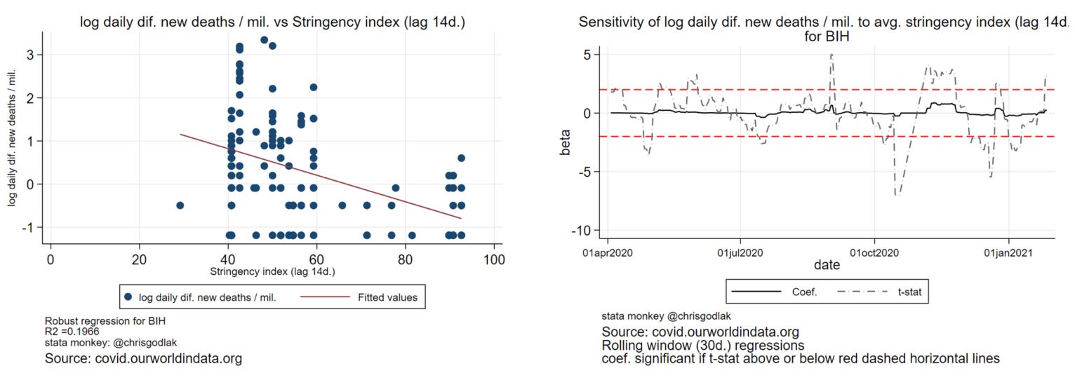
Bosnia has the largest negative coefficient from East Europe countries (i.e. NPI & deaths are negatively linked)
It has a negative slope and a 2 digits R² : 19.7%; meaning that almost 20% of the empirical observations can be “explained” with a linear adjustement
But over time beta is around 0, with > 0 and < 0 episodes; most significant are negative episodes in october and december (i.e. for these periods NPI & deaths are negatively linked), but we can also notice significant and positive episodes in september and november…
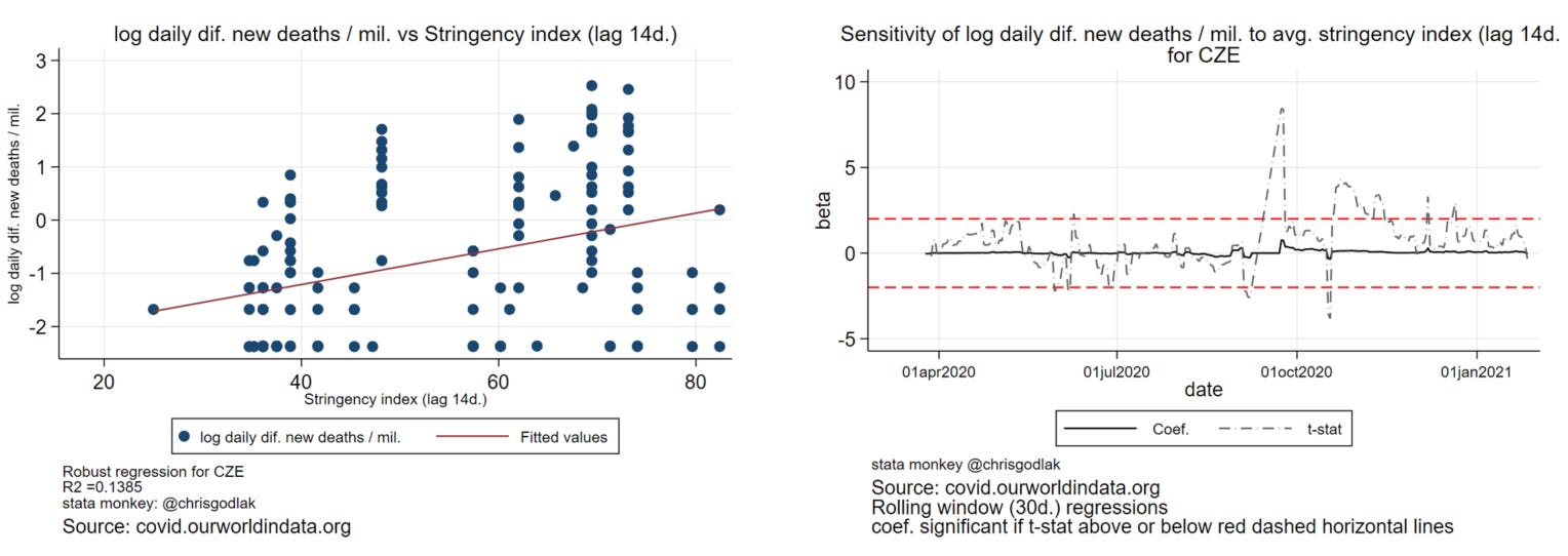
Czechia has the largest positive coefficient from East Europe (i.e. NPI & deaths are positively linked)
Positive slope and 2 digits R² at 13.9%; beta over time around 0 again with several positive episodes in fall, with a spike in september…
Let’s now turn to West Europe and pick the local champ with the largest > 0 coefficient (i.e. NPI & deaths are positively linked) : Germany !
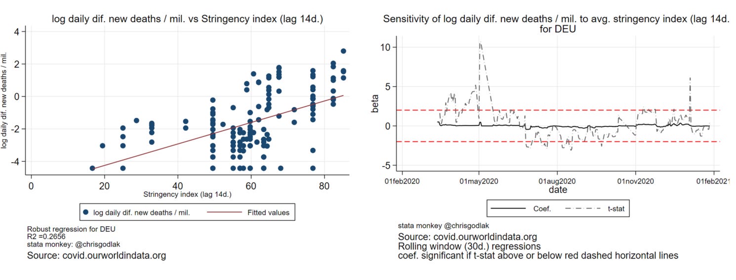
Positive slope with quite large R² at 26.6%; beta around 0 over time with significant and positive spikes in spring and in winter…
Let also bring into the pictures the next 2 champs: Italy and France
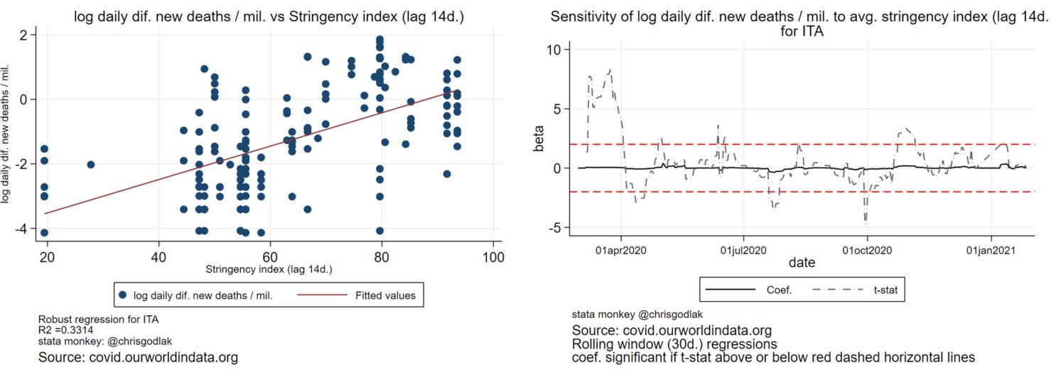
Italy: positive slope and even larger R² at 33.1% but again beta is around 0 over time, with a huge significant and positive spike in spring…
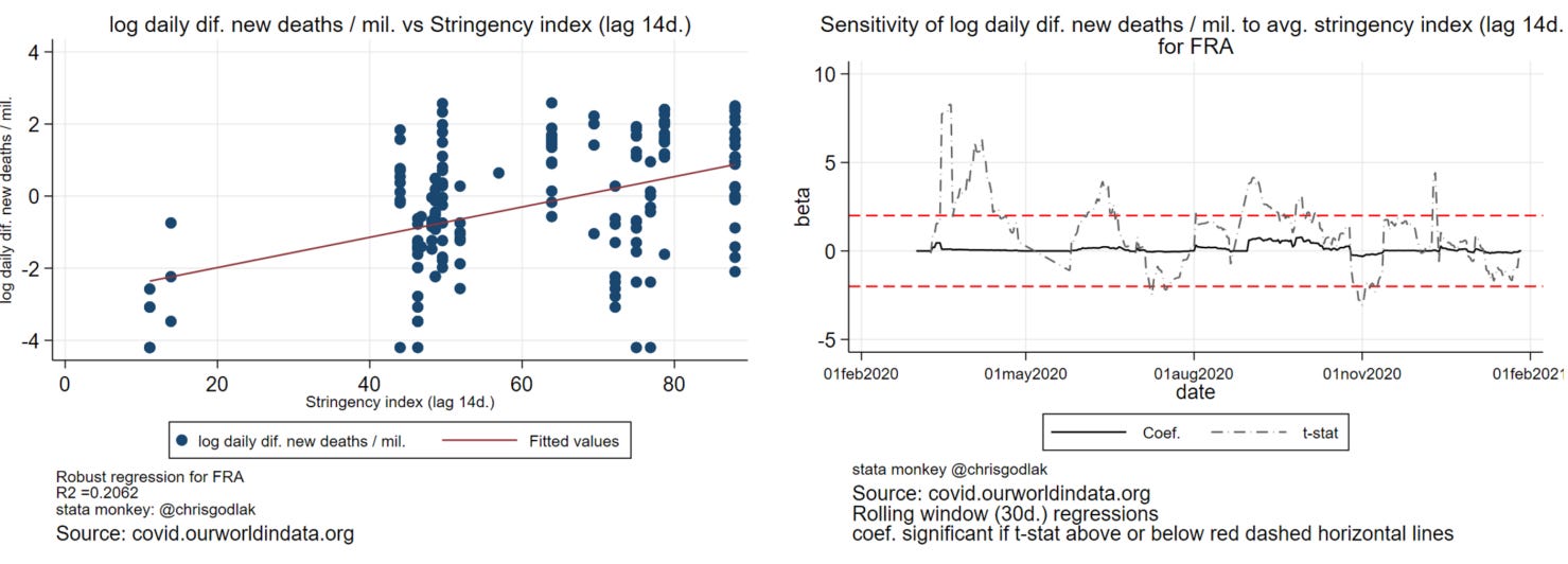
France: positive slope with R² at 20.6% and beta around 0 over time with a significant and positive spike in spring again…
I invite you to check all other available countries graphics under the link provided above
Overall, links between stringency & deaths are rather weak… except a few countries in Eastern Europe, the average link between stringency index (i.e. NPI) and deaths (log of daily variation in new deaths / million) is positive… And remember that stringency index is lagged by 14 days in the analysis… When we look into the evolution of this link over time (via rolling window regressions), it is mostly around 0 with some episods of significance; mostly in spring in West (and a positive link…)…
ADDENDUM Same excercise as above but without log smoothing for daily variation in new deaths / million and with a 30 days lagged stringency index
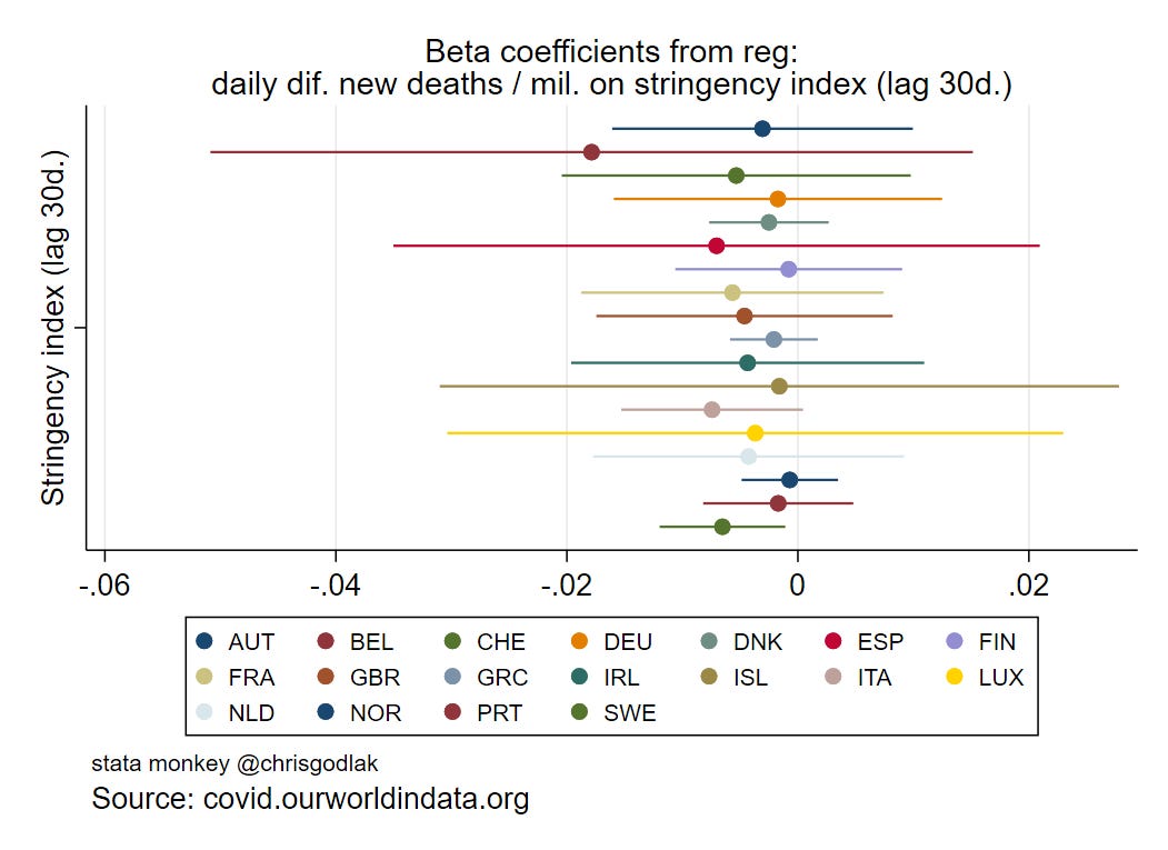
It seems things look even worse: coefficients around 0 (with large CI for some countries)
For consistency, i show again graphics for the same individual countries as above
All graphics are available under this link: https://icedrive.net/1/e2Be9K8h5J
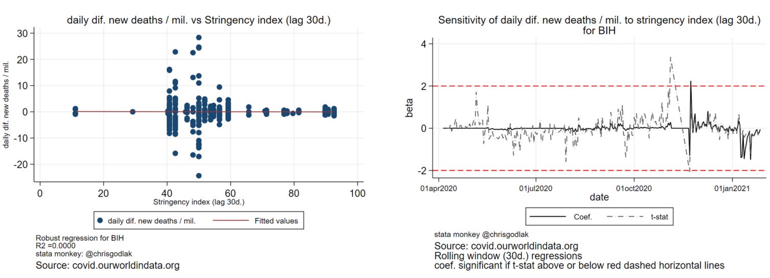
Bosnia: flat, R²=0, beta around 0 except for winter with some volatility, sometimes important, but not significant… one (positive !) peak significant in november…
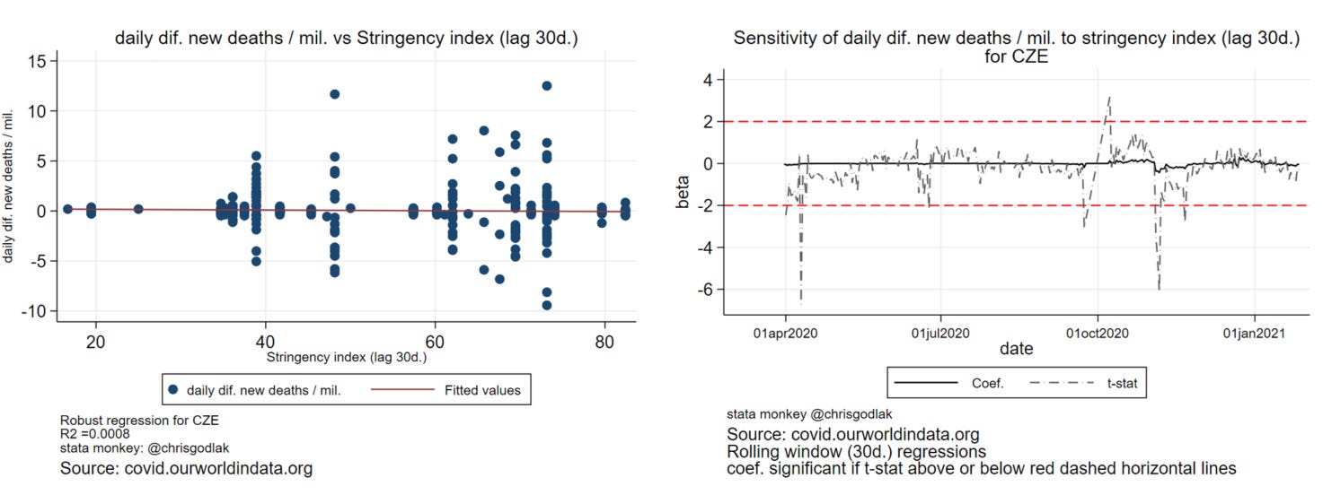
Czechia: flat, R²~0, beta around 0, only a few peaks with significance, some (large) negative in spring and fall…
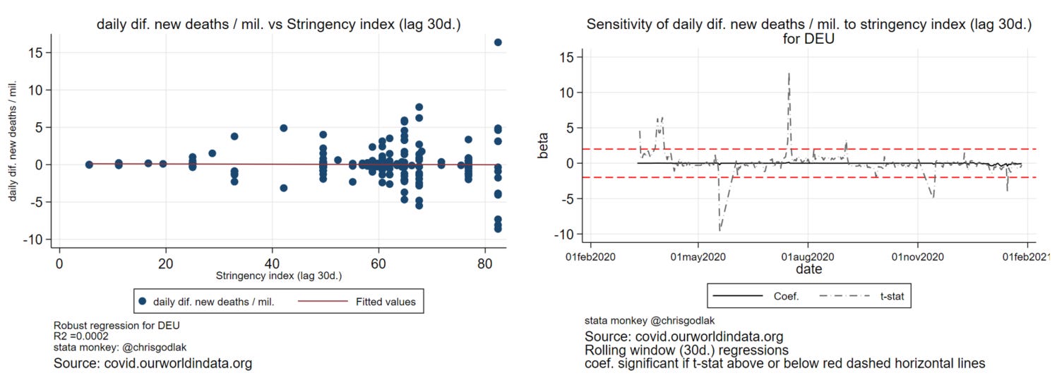
Germany: flat, R²~0, beta around 0, some peaks of significance, 1 in spring (negative), 1 in summer (positive !)…
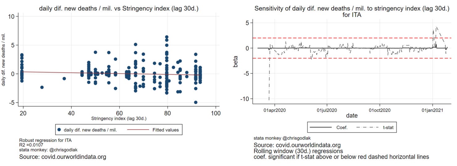
Italy: slighlty negative slope but R²~1%, beta around 0, 2 peaks; a negative one in early spring and a positive (!) one in winter…
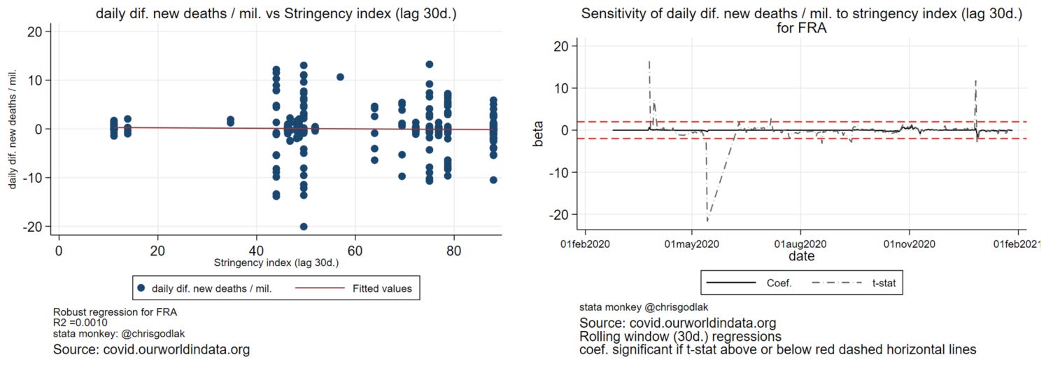
France: flat, R²~0, beta around 0; 3 major peaks: 2 positive (!) in early spring and late winter, 1 negative in late spring…
Overall, links between stringency & deaths are even worse when using non log variation in new deaths and lagging stringency by 30 days